> ## Documentation Index
> Fetch the complete documentation index at: https://docs.labelbox.com/llms.txt
> Use this file to discover all available pages before exploring further.
# Model run metrics
> A guide to understanding and navigating your automatically generated model run metrics in Labelbox.
Think of model metrics as a report card for your AI model. They help you understand how well your model is performing, where it's making mistakes, and how you can improve it. This guide will walk you through the essentials of using model metrics in Labelbox.
By analyzing your model's metrics, you can:
* **See what your model gets right and wrong**: Metrics help you identify correct predictions (true positives) and incorrect ones (false positives/negatives).
* **Find where your model is uncertain**: You can filter for low-confidence predictions to see where your model is struggling.
* **Improve your data quality**: By reviewing your model's mistakes, you might find errors in your ground truth labels.
* **Choose the best version of your model**: You can compare metrics across different model runs to see which one performs best.
Labelbox offers two types of metrics: **Automatic metrics** and **custom metrics**.
## Automatically generated metrics
Once you upload your model's predictions, Labelbox automatically calculates several key metrics. To get these automatic metrics, you need to have both predictions from your model and the correct answers (annotations or ground truth) in your dataset.
These metrics are computed on every feature and can be sorted and [filtered at the feature level](/docs/model-slices).
Automatic metrics are supported only for ontologies with fewer than 4,000 features. To learn more about these and other limits, see [Limits](https://docs.labelbox.com/docs/limits).
Key metrics explained:
| Metric | What it tells you |
| ----------------------------- | ------------------------------------------------------------------------------------------------------------------ |
| True postitive | Your model correctly predicted something that is actually there. |
| False positive | Your model predicted something that isn't actually there. |
| True negative | Your model correctly identified that something is not there. |
| False negative | Your model missed something that is actually there. |
| Precision | Of all the things your model predicted, how many were correct? |
| Recall | Of all the things that should have been predicted, how many did your model find? |
| F1 score | A single score that balances Precision and Recall. |
| Intersection over union (IoU) | For object detection, this measures how much a predicted bounding box overlaps with the ground truth bounding box. |
### The confusion matrix: A visual snapshot of performance
The confusion matrix is a powerful grid that gives you a quick, visual report card of your model's performance. It helps you instantly see where your model is succeeding and where it's getting confused.
**How to read the matrix**
* **Correct Predictions (The Diagonal):** Cells running from the top-left to the bottom-right show correct predictions (True Positives), where your model's predicted class matched the ground truth annotation. *Note: Predictions uploaded without a confidence score are automatically assigned a score of 1.*
* **Prediction Errors (Off-Diagonal):** All other cells highlight errors, showing where the model predicted the wrong class.
\*\*Find missed predictions and false alarms with \*\*`None`
The matrix includes a special `None` category to clearly identify key errors:
| `None` category | What it means | Type of error |
| --------------------------------- | ---------------------------------------------------------------------------- | -------------- |
| Prediction with `None` annotation | The model made a prediction that didn't correspond to any real annotation. | False positive |
| Annotation with `None` prediction | A real annotation existed, but the model failed to make a prediction for it. | Negative |
You can click on any cell in the matrix to instantly view the specific data examples that fall into that category, making it easy to investigate exactly what went right or wrong.
**How the matrix is built**
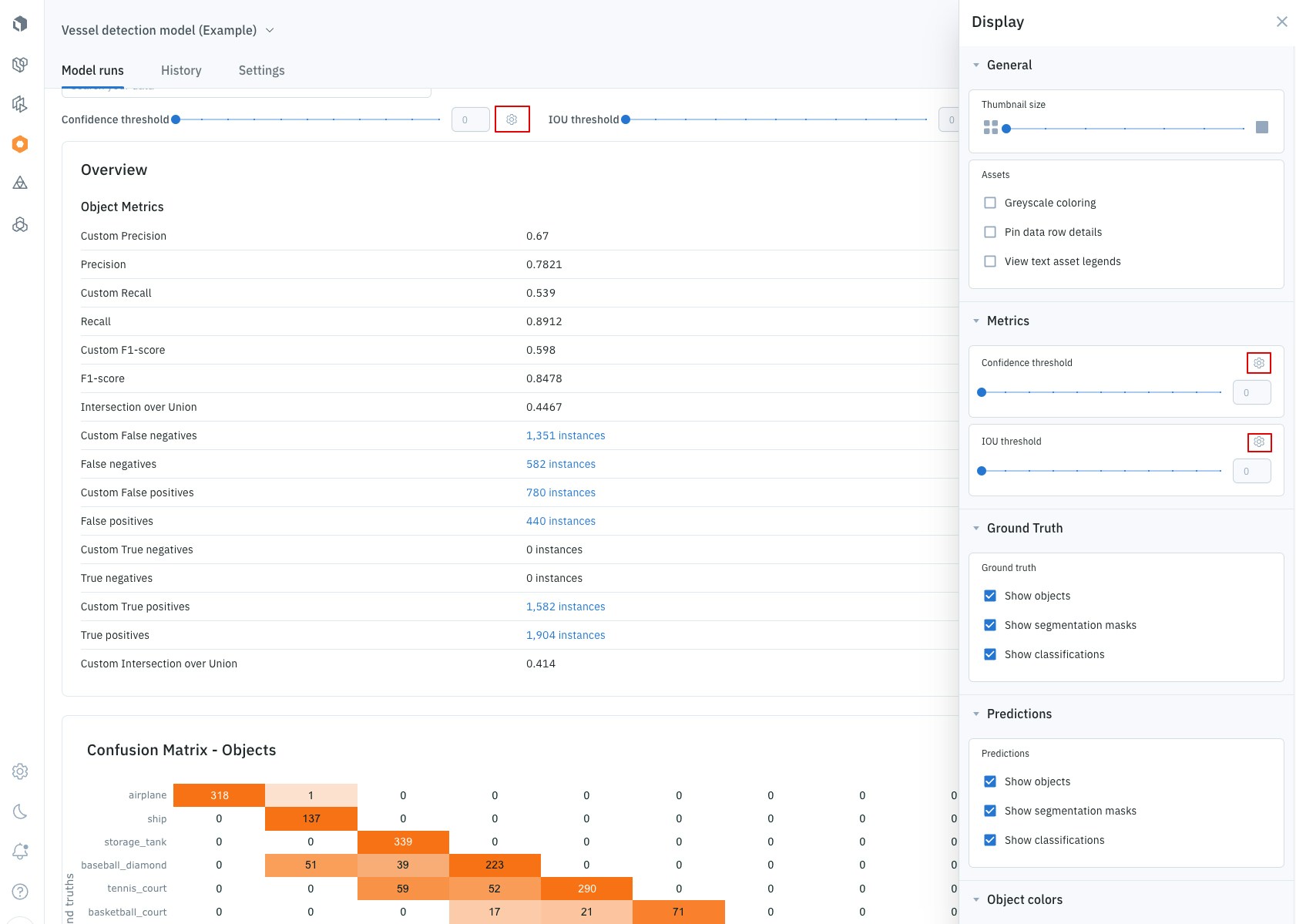
Labelbox generates the matrix by matching your model's predictions to the ground truth annotations. This matching process is governed by two thresholds you can control:
1. **Confidence Threshold:** First, it filters out any prediction with a confidence score below your selected value.
2. **IoU Threshold:** Then, it matches the remaining predictions to annotations based on their overlap (Intersection over Union, or IoU). A successful match must have an IoU score *above* this threshold.
Think of the **Confidence** and **IoU thresholds** as two main control knobs you can adjust to define what counts as a "correct" prediction for your model. Experimenting with these settings is key to understanding your model's performance and tuning it for your specific needs.
For classification models, you can still use the confusion matrix by setting the IoU threshold to `0`.
**Adjusting thresholds in Labelbox**
By default, you can instantly toggle between 11 standard values for both thresholds, from 0 to 1 in 0.1 increments.
* 11 values of confidence thresholds: 0, 0.1, 0.2, 0.3, ..., 0.7, 0.8, 0.9, 1
* 11 values of IoU thresholds: 0, 0.1, 0.2, 0.3, ..., 0.7, 0.8, 0.9, 1
As you adjust these values, you will see all your metrics and the confusion matrix update in real-time, helping you immediately see the impact.
Based on this matching, the system classifies every prediction as a True Positive, False Positive, or False Negative to populate the matrix.
If you need more granular control, you can easily customize the range of threshold values to focus on a specific area. For example, you can explore confidence values between 0.5 and 0.6 in tiny 0.01 steps.
1. Go to the **Display** panel.
2. Find the metric you want to adjust (e.g., Confidence or IoU) and click the **Settings** icon.
3. From there, you can add, remove, or edit the threshold values to create a custom range for your analysis.
 ### The precision-recall curve: Finding the right balance
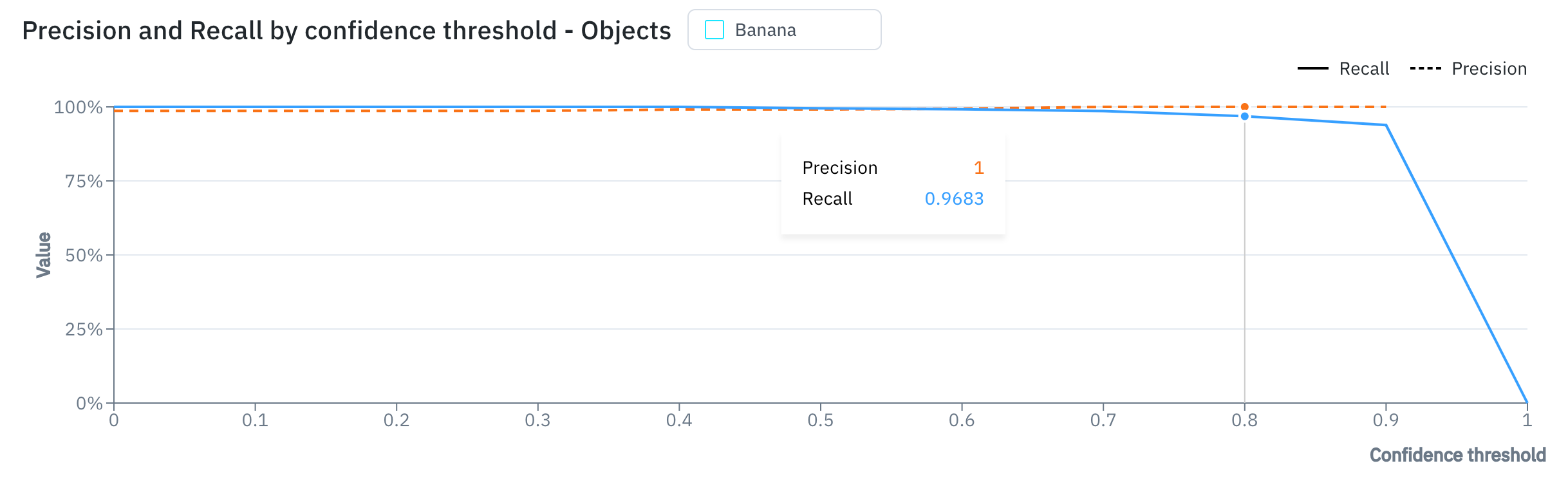
The **precision-recall curve** helps you decide on the best **confidence threshold** for your model. The confidence threshold is the minimum level of confidence your model needs to have before it makes a prediction.
* A **high** confidence threshold will result in fewer, but more accurate, predictions (high precision, low recall).
* A **low** confidence threshold will result in more predictions, but also more errors (low precision, high recall).
The curve helps you find the "sweet spot" that works best for your specific needs.
You can display the precision-recall curve for all features or a specific feature. This lets you choose the optimal confidence threshold for your use case for every class.
### The precision-recall curve: Finding the right balance
The **precision-recall curve** helps you decide on the best **confidence threshold** for your model. The confidence threshold is the minimum level of confidence your model needs to have before it makes a prediction.
* A **high** confidence threshold will result in fewer, but more accurate, predictions (high precision, low recall).
* A **low** confidence threshold will result in more predictions, but also more errors (low precision, high recall).
The curve helps you find the "sweet spot" that works best for your specific needs.
You can display the precision-recall curve for all features or a specific feature. This lets you choose the optimal confidence threshold for your use case for every class.
 ### View automatically generated model metrics
Follow these steps to view your model run metrics in the Labelbox UI:
1. Navigate to the **Model** tab in Labelbox.
2. Select your model run.
3. Use the **metrics view** to see a distribution of your metrics. You can compare metrics across different data slices or classes.
4. Switch to the **gallery view** to filter and sort your data based on metrics. This is a powerful way to find interesting examples, such as:
* Predictions with low confidence.
* Predictions that your model got wrong (false positives).
* Things your model missed (false negatives).
5. Click on any data row to see the detailed metrics for that specific prediction and annotation.
Automatic metrics may take a few minutes to calculate. Metric filters become available after metrics are generated. This means there can be a brief delay before metrics can be filtered.
## Custom metrics
If the automatic metrics aren't enough, you can use the Python SDK to create and [upload your own custom metrics](https://docs.labelbox.com/reference/model-run-custom-metrics). This is useful when you have specific things you want to measure that are unique to your project.
You can associate custom metrics with a variety of prediction or annotation types, including:
* Bounding boxes
* Checklists
* Free-form text
* Polygons
* And more...
### View custom metrics
To view custom metrics for a given data row:
1. Choose **Model** from the Labelbox main menu and then select the **Experiment** type.
2. Use the list of experiments to select the model run containing your custom metrics.
3. Select a data row to open Detail view.
4. Use the **Annotations** and **Predictions** panels to view custom metrics.
Once uploaded, you can use your custom metrics to [filter and sort your data](/docs/model-slices), just like with automatic metrics.
### View automatically generated model metrics
Follow these steps to view your model run metrics in the Labelbox UI:
1. Navigate to the **Model** tab in Labelbox.
2. Select your model run.
3. Use the **metrics view** to see a distribution of your metrics. You can compare metrics across different data slices or classes.
4. Switch to the **gallery view** to filter and sort your data based on metrics. This is a powerful way to find interesting examples, such as:
* Predictions with low confidence.
* Predictions that your model got wrong (false positives).
* Things your model missed (false negatives).
5. Click on any data row to see the detailed metrics for that specific prediction and annotation.
Automatic metrics may take a few minutes to calculate. Metric filters become available after metrics are generated. This means there can be a brief delay before metrics can be filtered.
## Custom metrics
If the automatic metrics aren't enough, you can use the Python SDK to create and [upload your own custom metrics](https://docs.labelbox.com/reference/model-run-custom-metrics). This is useful when you have specific things you want to measure that are unique to your project.
You can associate custom metrics with a variety of prediction or annotation types, including:
* Bounding boxes
* Checklists
* Free-form text
* Polygons
* And more...
### View custom metrics
To view custom metrics for a given data row:
1. Choose **Model** from the Labelbox main menu and then select the **Experiment** type.
2. Use the list of experiments to select the model run containing your custom metrics.
3. Select a data row to open Detail view.
4. Use the **Annotations** and **Predictions** panels to view custom metrics.
Once uploaded, you can use your custom metrics to [filter and sort your data](/docs/model-slices), just like with automatic metrics.